Plot returned point data

To launch this notebook interactively in a Jupyter notebook-like browser interface, please click the “Launch Binder” button below. Note that Binder may take several minutes to launch.

This notebook provides some examples for how to use matplotlib to plot the data returned from hf_hydrodata’s get_point_data function.

Please see the full point module documentation for information on what data is available, our data collection process, and new features we are working on! Our Metadata Description page itemizes the fields that get returned from get_point_metadata.

# Import packages
from hf_hydrodata import register_api_pin, get_point_data, get_point_metadata
from matplotlib import pyplot as plt
import pandas as pd

# You need to register on https://hydrogen.princeton.edu/pin
# and run the following with your registered information
# before you can use the hydrodata utilities
register_api_pin("your_email", "your_pin")

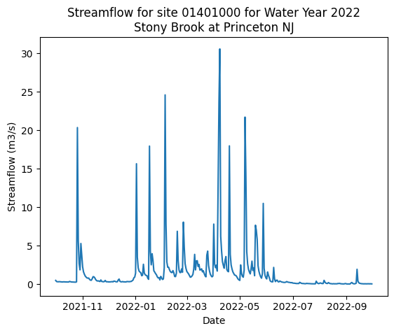
Example 1: Plot data for a single site location for one Water Year

In this example, we are going to work with daily streamflow data. However all non-instantaneous data is returned in the same format so this code is transferrable to other types of data requests.

# Set our site_id
site_id = "01401000"

# Request data and set the 'date' field to be the index
data_df = get_point_data(dataset="usgs_nwis", variable="streamflow", temporal_resolution="daily", aggregation="mean",
                         site_ids=site_id,
                         date_start="2021-10-01", date_end="2022-09-30").set_index('date')

# Set the index to data type 'datetime'
data_df.index = pd.to_datetime(data_df.index)

# Browse returned DataFrame
data_df

	01401000
date
2021-10-01	0.495250
2021-10-02	0.345260
2021-10-03	0.325450
2021-10-04	0.316960
2021-10-05	0.333940
...	...
2022-09-26	0.061694
2022-09-27	0.049808
2022-09-28	0.058864
2022-09-29	0.050657
2022-09-30	0.046129

365 rows × 1 columns

# Request metadata using the same query parameters to get this site's site name
metadata_df = get_point_metadata(dataset="usgs_nwis", variable="streamflow", temporal_resolution="daily", aggregation="mean",
                                 site_ids=site_id)

site_name = metadata_df.loc[metadata_df["site_id"] == site_id, "site_name"][0]
print(f"Site name: {site_name}")

# Set units
units = "m3/s"

Site name: Stony Brook at Princeton NJ

# Plot
plt.plot(data_df)
plt.xlabel("Date")
plt.ylabel(f"Streamflow ({units})")
plt.title(f'Streamflow for site {site_id} for Water Year 2022\n{site_name}')

plt.show()

# If you want to save a version, uncomment the following with your desired file path
# plt.savefig(f'path/to/save/streamflow_{site_id}.png')

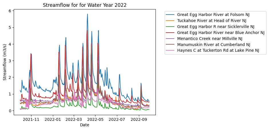
Example 2: Plot data for all locations within a bounding box for one Water Year

# Specify latitude/longitude bounding box
latitude_range = (39, 40)
longitude_range = (-75, -74.8)

# Request data
data_df = get_point_data(dataset="usgs_nwis", variable="streamflow",
                         temporal_resolution="daily", aggregation="mean",
                         date_start="2021-10-01", date_end="2022-09-30",
                         latitude_range=latitude_range, longitude_range=longitude_range).set_index('date')

# Set the index to data type 'datetime'
data_df.index = pd.to_datetime(data_df.index)

# Request metadata to get site names
metadata_df = get_point_metadata(dataset="usgs_nwis", variable="streamflow",
                                 temporal_resolution="daily", aggregation="mean",
                                 date_start="2021-10-01", date_end="2022-09-30",
                                 latitude_range=latitude_range, longitude_range=longitude_range)

site_ids_data = list(data_df.columns)
site_ids_metadata = list(metadata_df['site_id'])
assert site_ids_data == site_ids_metadata

# Set units
units = "m3/s"

# Plot
plt.plot(data_df)
plt.xlabel("Date")
plt.ylabel(f"Streamflow ({units})")
plt.title(f"Streamflow for for Water Year 2022")

# Create a legend of corresponding site names
# (remove or adjust the bbox_to_anchor parameter to move legend around)
site_names = metadata_df['site_name']
plt.legend(site_names, bbox_to_anchor=(1.05, 1))

plt.show()

# If you want to save a version, uncomment the following with your desired file path
# plt.savefig(f'path/to/save/streamflow.png')